Algorithmic drawing
Shaping functions
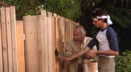
This chapter could be named "Mr. Miyagi's fence lesson." Previously, we mapped the normalized position of x and y to the red and green channels. Essentially we made a function that takes a two dimensional vector (x and y) and returns a four dimensional vector (r, g, b and a). But before we go further transforming data between dimensions we need to start simpler... much simpler. That means understanding how to make one dimensional functions. The more energy and time you spend learning and mastering this, the stronger your shader karate will be.
The following code structure is going to be our fence. In it, we visualize the normalized value of the x coordinate (st.x) in two ways: one with brightness (observe the nice gradient from black to white) and the other by plotting a green line on top (in that case the x value is assigned directly to y). Don't focus too much on the plot function, we will go through it in more detail in a moment.
Quick Note: The vec3 type constructor "understands" that you want to assign the three color channels with the same value, while vec4 understands that you want to construct a four dimensional vector with a three dimensional one plus a fourth value (in this case the value that controls the alpha or opacity). See for example lines 19 and 25 above.
This code is your fence; it's important to observe and understand it. You will come back over and over to this space between 0.0 and 1.0. You will master the art of blending and shaping this line.
This one-to-one relationship between x and y (or the brightness) is known as linear interpolation. From here we can use some mathematical functions to shape the line. For example we can raise x to the power of 5 to make a curved line.
Interesting, right? On line 22 try different exponents: 20.0, 2.0, 1.0, 0.0, 0.2 and 0.02 for example. Understanding this relationship between the value and the exponent will be very helpful. Using these types of mathematical functions here and there will give you expressive control over your code, a sort of data acupuncture that let you control the flow of values.
pow() is a native function in GLSL and there are many others. Most of them are accelerated at the level of the hardware, which means if they are used in the right way and with discretion they will make your code faster.
Replace the power function on line 22. Try other ones like: exp(), log() and sqrt(). Some of these functions are more interesting when you play with them using PI. You can see on line 8 that I have defined a macro that will replace any use of PI with the value 3.14159265359.
Step and Smoothstep
GLSL also has some unique native interpolation functions that are hardware accelerated.
The step() interpolation receives two parameters. The first one is the limit or threshold, while the second one is the value we want to check or pass. Any value under the limit will return 0.0 while everything above the limit will return 1.0.
Try changing this threshold value on line 20 of the following code.
The other unique function is known as smoothstep(). Given a range of two numbers and a value, this function will interpolate the value between the defined range. The two first parameters are for the beginning and end of the transition, while the third is for the value to interpolate.
In the previous example, on line 12, notice that we’ve been using smoothstep to draw the green line on the plot() function. For each position along the x axis this function makes a bump at a particular value of y. How? By connecting two smoothstep() together. Take a look at the following function, replace it for line 20 above and think of it as a vertical cut. The background does look like a line, right?
float y = smoothstep(0.2,0.5,st.x) - smoothstep(0.5,0.8,st.x);Sine and Cosine
When you want to use some math to animate, shape or blend values, there is nothing better than being friends with sine and cosine.
These two basic trigonometric functions work together to construct circles that are as handy as MacGyver’s Swiss army knife. It’s important to know how they behave and in what ways they can be combined. In a nutshell, given an angle (in radians) they will return the correct position of x (cosine) and y (sine) of a point on the edge of a circle with a radius equal to 1. But, the fact that they return normalized values (values between -1 and 1) in such a smooth way makes them an incredible tool.
While it's difficult to describe all the relationships between trigonometric functions and circles, the above animation does a beautiful job of visually summarizing these relationships.
Take a careful look at this sine wave. Note how the y values flow smoothly between +1 and -1. As we saw in the time example in the previous chapter, you can use this rhythmic behavior of sin() to animate properties. If you are reading this example in a browser you will see that you can change the code in the formula above to watch how the wave changes. (Note: don't forget the semicolon at the end of the lines.)
Try the following exercises and notice what happens:
-
Add time (
u_time) to x before computing thesin. Internalize that motion along x. -
Multiply x by
PIbefore computing thesin. Note how the two phases shrink so each cycle repeats every 2 integers. -
Multiply time (
u_time) by x before computing thesin. See how the frequency between phases becomes more and more compressed. Note that u_time may have already become very large, making the graph hard to read. -
Add 1.0 to
sin(x). See how all the wave is displaced up and now all values are between 0.0 and 2.0. -
Multiply
sin(x)by 2.0. See how the amplitude doubles in size. -
Compute the absolute value (
abs()) ofsin(x). It looks like the trace of a bouncing ball. -
Extract just the fraction part (
fract()) of the resultant ofsin(x). - Add the higher integer (
ceil()) and the smaller integer (floor()) of the resultant ofsin(x)to get a digital wave of 1 and -1 values.
Some extra useful functions
At the end of the last exercise we introduced some new functions. Now it’s time to experiment with each one by uncommenting the lines below one at a time. Get to know these functions and study how they behave. I know, you are wondering... why? A quick google search on "generative art" will tell you. Keep in mind that these functions are our fence. We are mastering the movement in one dimension, up and down. Soon, it will be time for two, three and four dimensions!

Advance shaping functions
Golan Levin has great documentation of more complex shaping functions that are extraordinarily helpful. Porting them to GLSL is a really smart move, to start building your own resource of snippets of code.
-
Polynomial Shaping Functions: www.flong.com/archive/texts/code/shapers_poly
-
Exponential Shaping Functions: www.flong.com/archive/texts/code/shapers_exp
-
Circular & Elliptical Shaping Functions: www.flong.com/archive/texts/code/shapers_circ
- Bezier and Other Parametric Shaping Functions: www.flong.com/archive/texts/code/shapers_bez
Like chefs that collect spices and exotic ingredients, digital artists and creative coders have a particular love of working on their own shaping functions.
Iñigo Quiles has a great collection of useful functions. After reading this article take a look at the following translation of these functions to GLSL. Pay attention to the small changes required, like putting the "." (dot) on floating point numbers and using the GLSL name for C functions; for example instead of powf() use pow():
To keep your motivation up, here is an elegant example (made by Danguafer) of mastering the shaping-functions karate.
In the Next >> chapter we will start using our new moves. First with mixing colors and then drawing shapes.
Exercise
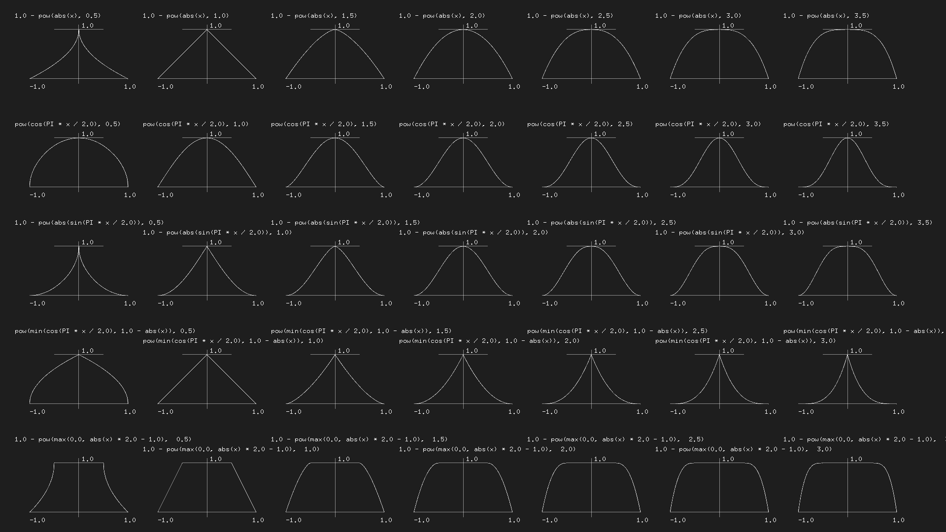
Take a look at the following table of equations made by Kynd. See how he is combining functions and their properties to control the values between 0.0 and 1.0. Now it's time for you to practice by replicating these functions. Remember the more you practice the better your karate will be.
For your toolbox
-
LYGIA is a shader library of reusable functions that can be include easily on your projects. It's very granular, designed for reusability, performance and flexibility. And can be easily be added to any projects and frameworks. It's divided in different sections and it have an entire one formath operations
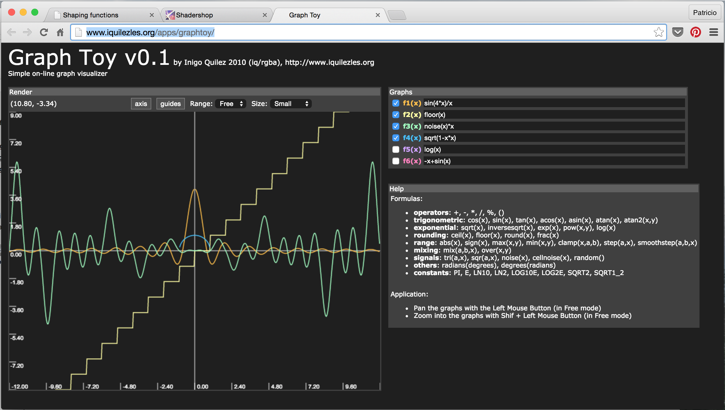
- GraphToy: once again Iñigo Quilez made a tool to visualize GLSL functions in WebGL.