Shapes

Finally! We have been building skills for this moment! You have learned most of the GLSL foundations, types and functions. You have practiced your shaping equations over and over. Now is the time to put it all together. You are up for this challenge! In this chapter you'll learn how to draw simple shapes in a parallel procedural way.

Rectangle

Imagine we have grid paper like we used in math classes and our homework is to draw a square. The paper size is 10x10 and the square is supposed to be 8x8. What will you do?

You'd paint everything except the first and last rows and the first and last column, right?

How does this relate to shaders? Each little square of our grid paper is a thread (a pixel). Each little square knows its position, like the coordinates of a chess board. In previous chapters we mapped x and y to the red and green color channels, and we learned how to use the narrow two dimensional territory between 0.0 and 1.0. How can we use this to draw a centered square in the middle of our billboard?

Let's start by sketching pseudocode that uses if statements over the spatial field. The principles to do this are remarkably similar to how we think of the grid paper scenario.

if ( (X GREATER THAN 1) AND (Y GREATER THAN 1) )
    paint white
else
    paint black

Now that we have a better idea of how this will work, let’s replace the if statement with step(), and instead of using 10x10 let’s use normalized values between 0.0 and 1.0:

uniform vec2 u_resolution;

void main(){
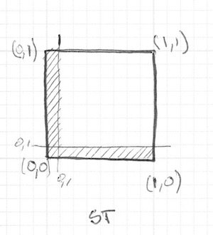
    vec2 st = gl_FragCoord.xy/u_resolution.xy;
    vec3 color = vec3(0.0);

    // Each result will return 1.0 (white) or 0.0 (black).
    float left = step(0.1,st.x);   // Similar to ( X greater than 0.1 )
    float bottom = step(0.1,st.y); // Similar to ( Y greater than 0.1 )

    // The multiplication of left*bottom will be similar to the logical AND.
    color = vec3( left * bottom );

    gl_FragColor = vec4(color,1.0);
}

The step() function will turn every pixel below 0.1 to black (vec3(0.0)) and the rest to white (vec3(1.0)) . The multiplication between left and bottom works as a logical AND operation, where both must be 1.0 to return 1.0 . This draws two black lines, one on the bottom and the other on the left side of the canvas.

In the previous code we repeat the structure for each axis (left and bottom). We can save some lines of code by passing two values directly to step() instead of one. That looks like this:

vec2 borders = step(vec2(0.1),st);
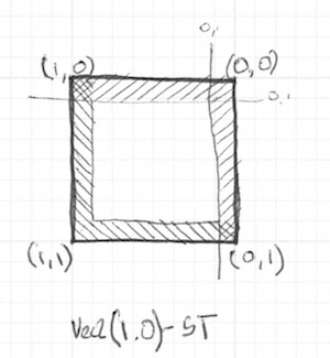
float pct = borders.x * borders.y;

So far, we’ve only drawn two borders (bottom-left) of our rectangle. Let's do the other two (top-right). Check out the following code:

Uncomment lines 21-22 and see how we invert the st coordinates and repeat the same step() function. That way the vec2(0.0,0.0) will be in the top right corner. This is the digital equivalent of flipping the page and repeating the previous procedure.

Take note that in lines 18 and 22 all of the sides are being multiplied together. This is equivalent to writing:

vec2 bl = step(vec2(0.1),st);       // bottom-left
vec2 tr = step(vec2(0.1),1.0-st);   // top-right
color = vec3(bl.x * bl.y * tr.x * tr.y);

Interesting right? This technique is all about using step() and multiplication for logical operations and flipping the coordinates.

Before going forward, try the following exercises:

• Change the size and proportions of the rectangle.

• Experiment with the same code but using smoothstep() instead of step(). Note that by changing values, you can go from blurred edges to elegant smooth borders.

• Do another implementation that uses floor().

• Choose the implementation you like the most and make a function of it that you can reuse in the future. Make your function flexible and efficient.

• Make another function that just draws the outline of a rectangle.

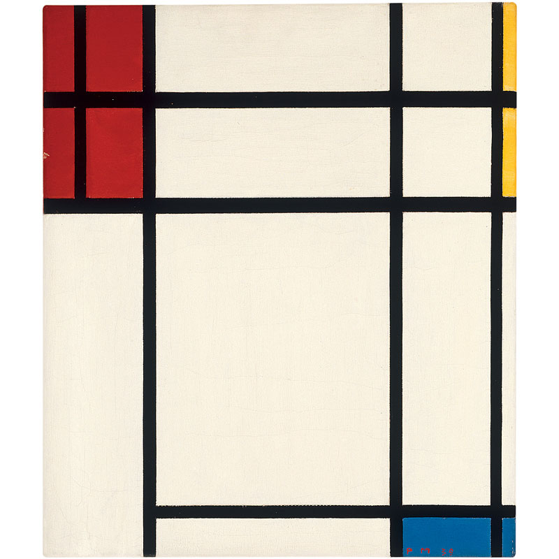
• How do you think you can move and place different rectangles in the same billboard? If you figure out how, show off your skills by making a composition of rectangles and colors that resembles a Piet Mondrian painting.

Circles

It's easy to draw squares on grid paper and rectangles on cartesian coordinates, but circles require another approach, especially since we need a "per-pixel" algorithm. One solution is to re-map the spatial coordinates so that we can use a step() function to draw a circle.

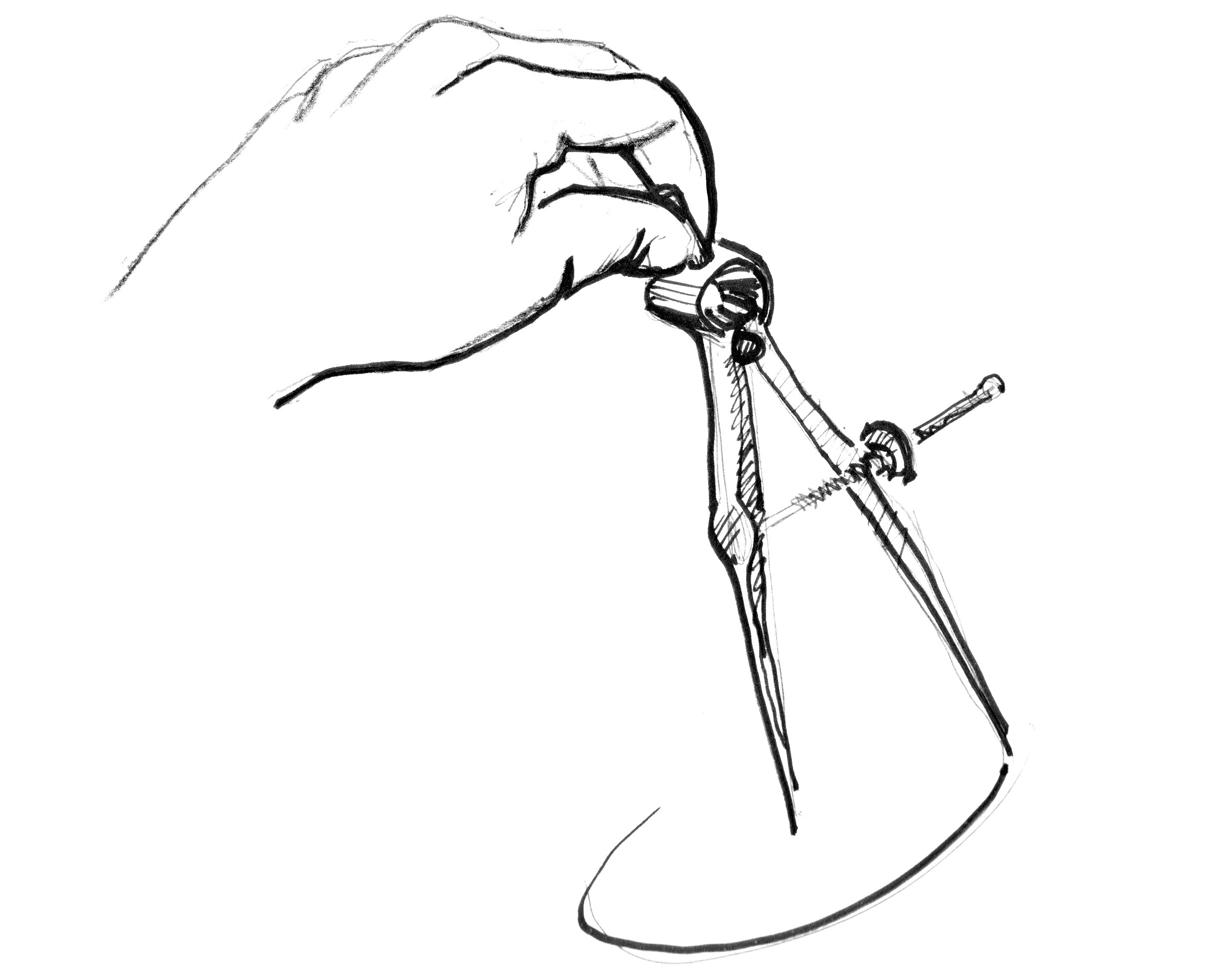
How? Let's start by going back to math class and the grid paper, where we opened a compass to the radius of a circle, pressed one of the compass points at the center of the circle and then traced the edge of the circle with a simple spin.

Translating this to a shader where each square on the grid paper is a pixel implies asking each pixel (or thread) if it is inside the area of the circle. We do this by computing the distance from the pixel to the center of the circle.

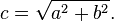
There are several ways to calculate that distance. The easiest one uses the distance() function, which internally computes the length() of the difference between two points (in our case the pixel coordinate and the center of the canvas). The length() function is nothing but a shortcut of the hypotenuse equation that uses square root (sqrt()) internally.

You can use distance(), length() or sqrt() to calculate the distance to the center of the billboard. The following code contains these three functions and the non-surprising fact that each one returns exactly same result.

• Comment and uncomment lines to try the different ways to get the same result.

In the previous example we map the distance to the center of the billboard to the color brightness of the pixel. The closer a pixel is to the center, the lower (darker) value it has. Notice that the values don't get too high because from the center ( vec2(0.5, 0.5) ) the maximum distance barely goes over 0.5. Contemplate this map and think:

• What you can infer from it?

• How we can use this to draw a circle?

• Modify the above code in order to contain the entire circular gradient inside the canvas.

Distance field

We can also think of the above example as an altitude map, where darker implies taller. The gradient shows us something similar to the pattern made by a cone. Imagine yourself on the top of that cone. The horizontal distance to the edge of the cone is 0.5. This will be constant in all directions. By choosing where to “cut” the cone you will get a bigger or smaller circular surface.

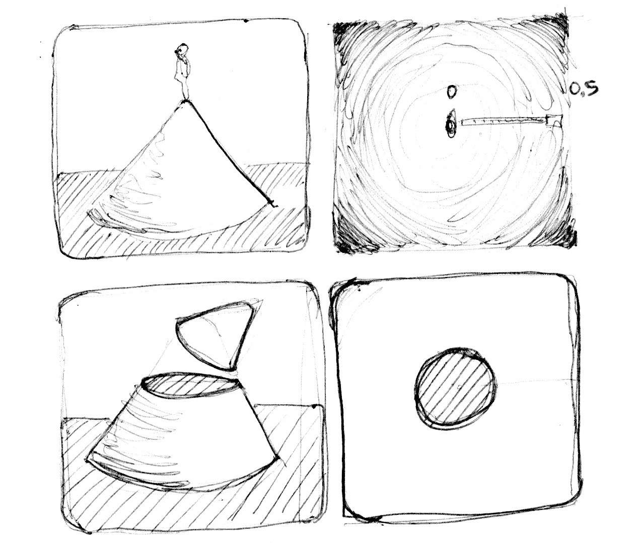
Basically we are using a re-interpretation of the space (based on the distance to the center) to make shapes. This technique is known as a “distance field” and is used in different ways from font outlines to 3D graphics.

Try the following exercises:

• Use step() to turn everything above 0.5 to white and everything below to 0.0.

• Inverse the colors of the background and foreground.

• Using smoothstep(), experiment with different values to get nice smooth borders on your circle.

• Once you are happy with an implementation, make a function of it that you can reuse in the future.

• Add color to the circle.

• Can you animate your circle to grow and shrink, simulating a beating heart? (You can get some inspiration from the animation in the previous chapter.)

• What about moving this circle? Can you move it and place different circles in a single billboard?

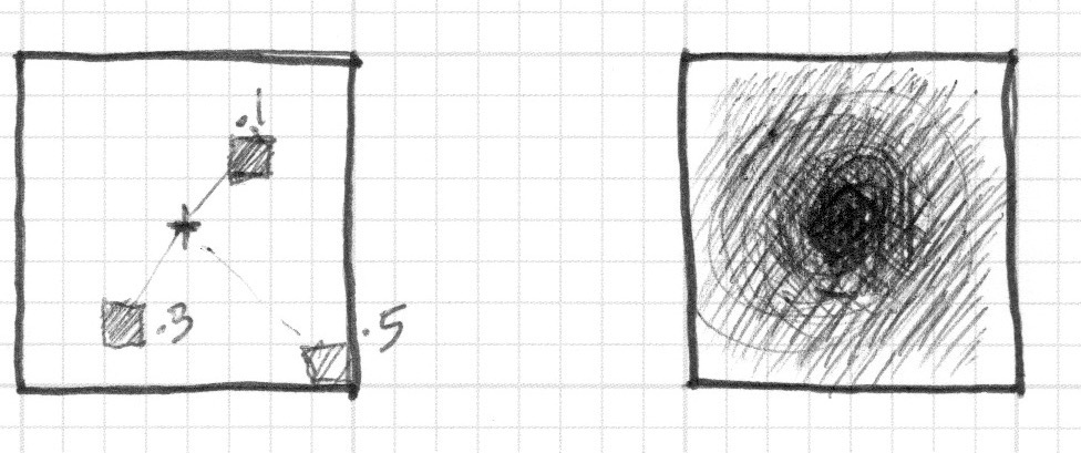
• What happens if you combine distances fields together using different functions and operations?

pct = distance(st,vec2(0.4)) + distance(st,vec2(0.6));
pct = distance(st,vec2(0.4)) * distance(st,vec2(0.6));
pct = min(distance(st,vec2(0.4)),distance(st,vec2(0.6)));
pct = max(distance(st,vec2(0.4)),distance(st,vec2(0.6)));
pct = pow(distance(st,vec2(0.4)),distance(st,vec2(0.6)));

• Make three compositions using this technique. If they are animated, even better!

For your tool box

In terms of computational power the sqrt() function - and all the functions that depend on it - can be expensive. Here is another way to create a circular distance field by using dot() product.

Useful properties of a Distance Field

Distance fields can be used to draw almost everything. Obviously the more complex a shape is, the more complicated its equation will be, but once you have the formula to make distance fields of a particular shape it is very easy to combine and/or apply effects to it, like smooth edges and multiple outlines. Because of this, distance fields are popular in font rendering, like Mapbox GL Labels, Matt DesLauriers Material Design Fonts and as is described on Chapter 7 of iPhone 3D Programming, O’Reilly.

Take a look at the following code.

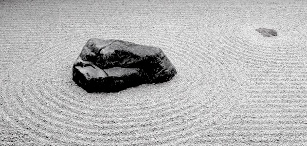
We start by moving the coordinate system to the center and shrinking it in half in order to remap the position values between -1 and 1. Also on line 24 we are visualizing the distance field values using a fract() function making it easy to see the pattern they create. The distance field pattern repeats over and over like rings in a Zen garden.

Let’s take a look at the distance field formula on line 19. There we are calculating the distance to the position on (.3,.3) or vec3(.3) in all four quadrants (that’s what abs() is doing there).

If you uncomment line 20, you will note that we are combining the distances to these four points using the min() to zero. The result produces an interesting new pattern.

Now try uncommenting line 21; we are doing the same but using the max() function. The result is a rectangle with rounded corners. Note how the rings of the distance field get smoother the further away they get from the center.

Finish uncommenting lines 27 to 29 one by one to understand the different uses of a distance field pattern.

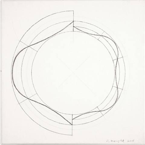
Polar shapes

In the chapter about color we map the cartesian coordinates to polar coordinates by calculating the radius and angles of each pixel with the following formula:

vec2 pos = vec2(0.5)-st;
float r = length(pos)*2.0;
float a = atan(pos.y,pos.x);

We use part of this formula at the beginning of the chapter to draw a circle. We calculated the distance to the center using length(). Now that we know about distance fields we can learn another way of drawing shapes using polar coordinates.

This technique is a little restrictive but very simple. It consists of changing the radius of a circle depending on the angle to achieve different shapes. How does the modulation work? Yes, using shaping functions!

Below you will find the same functions in the cartesian graph and in a polar coordinates shader example (between lines 21 and 25). Uncomment the functions one-by-one, paying attention the relationship between one coordinate system and the other.

Try to:

• Animate these shapes.
• Combine different shaping functions to cut holes in the shape to make flowers, snowflakes and gears.
• Use the plot() function we were using in the Shaping Functions Chapter to draw just the contour.

Combining powers

Now that we've learned how to modulate the radius of a circle according to the angle using the atan() to draw different shapes, we can learn how use atan() with distance fields and apply all the tricks and effects possible with distance fields.

The trick will use the number of edges of a polygon to construct the distance field using polar coordinates. Check out the following code from Andrew Baldwin.

• Using this example, make a function that inputs the position and number of corners of a desired shape and returns a distance field value.

• Mix distance fields together using min() and max().

• Choose a geometric logo to replicate using distance fields.

Congratulations! You have made it through the rough part! Take a break and let these concepts settle - drawing simple shapes in Processing is easy but not here. In shader-land drawing shapes is twisted, and it can be exhausting to adapt to this new paradigm of coding.

For your toolbox

• LYGIA's draw functions are set of reusable functions to draw 2D shapes and patterns. You can also explore LYGIA's SDF functions folder to combine more complex shapes through distance fields. It's very granular library, designed for reusability, performance and flexibility. And it can be easily be added to any projects and frameworks.

• Down at the end of this chapter you will find a link to PixelSpirit Deck this deck of cards will help you learn new SDF functions, compose them into your designs and use on your shaders. The deck has a progressive learning curve, so taking one card a day and working on it will push and challenge your skills for months.

Now that you know how to draw shapes I'm sure new ideas will pop into your mind. In the following chapter you will learn how to move, rotate and scale shapes. This will allow you to make compositions!