Noise

It's time for a break! We've been playing with random functions that look like TV white noise, our head is still spinning thinking about shaders, and our eyes are tired. Time to go out for a walk!

We feel the air on our skin, the sun in our face. The world is such a vivid and rich place. Colors, textures, sounds. While we walk we can't avoid noticing the surface of the roads, rocks, trees and clouds.

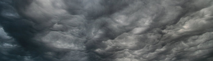
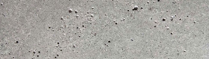
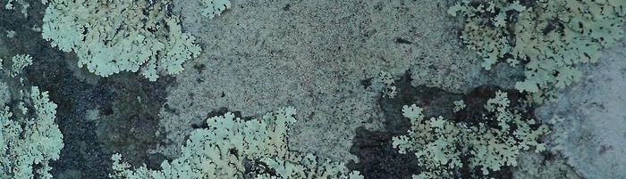
The unpredictability of these textures could be called "random," but they don't look like the random we were playing with before. The “real world” is such a rich and complex place! How can we approximate this variety computationally?

This was the question Ken Perlin was trying to solve in the early 1980s when he was commissioned to generate more realistic textures for the movie "Tron." In response to that, he came up with an elegant Oscar winning noise algorithm. (No biggie.)

The following is not the classic Perlin noise algorithm, but it is a good starting point to understand how to generate noise.

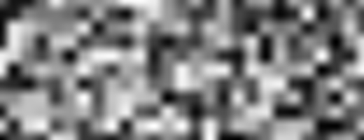
In these lines we are doing something similar to what we did in the previous chapter. We are subdividing a continuous floating number (x) into its integer (i) and fractional (f) components. We use floor() to obtain i and fract() to obtain f. Then we apply rand() to the integer part of x, which gives a unique random value for each integer.

After that you see two commented lines. The first one interpolates each random value linearly.

y = mix(rand(i), rand(i + 1.0), f);

Go ahead and uncomment this line to see how this looks. We use the fract() value store in f to mix() the two random values.

At this point in the book, we've learned that we can do better than a linear interpolation, right? Now try uncommenting the following line, which uses a smoothstep() interpolation instead of a linear one.

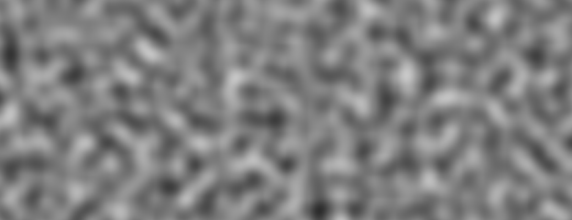
y = mix(rand(i), rand(i + 1.0), smoothstep(0.,1.,f));

After uncommenting it, notice how the transition between the peaks gets smooth. In some noise implementations you will find that programmers prefer to code their own cubic curves (like the following formula) instead of using the smoothstep().

float u = f * f * (3.0 - 2.0 * f ); // custom cubic curve
y = mix(rand(i), rand(i + 1.0), u); // using it in the interpolation

This smooth randomness is a game changer for graphical engineers or artists - it provides the ability to generate images and geometries with an organic feeling. Perlin's Noise Algorithm has been implemented over and over in different languages and dimensions to make mesmerizing pieces for all sorts of creative uses.

Now it's your turn:

• Make your own float noise(float x) function.

• Use your noise function to animate a shape by moving it, rotating it or scaling it.

• Make an animated composition of several shapes 'dancing' together using noise.

• Construct "organic-looking" shapes using the noise function.

• Once you have your "creature," try to develop it further into a character by assigning it a particular movement.

2D Noise

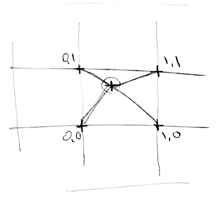
Now that we know how to do noise in 1D, it's time to move on to 2D. In 2D, instead of interpolating between two points of a line (rand(x) and rand(x)+1.0), we are going to interpolate between the four corners of the square area of a plane (rand(st), rand(st)+vec2(1.,0.), rand(st)+vec2(0.,1.) and rand(st)+vec2(1.,1.)).

Similarly, if we want to obtain 3D noise we need to interpolate between the eight corners of a cube. This technique is all about interpolating random values, which is why it's called value noise.

Like the 1D example, this interpolation is not linear but cubic, which smoothly interpolates any points inside our square grid.

Take a look at the following noise function.

We start by scaling the space by 5 (line 45) in order to see the interpolation between the squares of the grid. Then inside the noise function we subdivide the space into cells. We store the integer position of the cell along with the fractional positions inside the cell. We use the integer position to calculate the four corners' coordinates and obtain a random value for each one (lines 23-26). Finally, in line 35 we interpolate between the 4 random values of the corners using the fractional positions we stored before.

Now it's your turn. Try the following exercises:

• Change the multiplier of line 45. Try to animate it.

• At what level of zoom does the noise start looking like random again?

• At what zoom level is the noise is imperceptible?

• Try to hook up this noise function to the mouse coordinates.

• What if we treat the gradient of the noise as a distance field? Make something interesting with it.

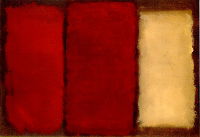
• Now that you've achieved some control over order and chaos, it's time to use that knowledge. Make a composition of rectangles, colors and noise that resembles some of the complexity of a Mark Rothko painting.

Using Noise in Generative Designs

Noise algorithms were originally designed to give a natural je ne sais quoi to digital textures. The 1D and 2D implementations we've seen so far were interpolations between random values, which is why they're called Value Noise, but there are more ways to obtain noise...

As you discovered in the previous exercises, value noise tends to look "blocky." To diminish this blocky effect, in 1985 Ken Perlin developed another implementation of the algorithm called Gradient Noise. Ken figured out how to interpolate random gradients instead of values. These gradients were the result of a 2D random function that returns directions (represented by a vec2) instead of single values (float). Click on the following image to see the code and how it works.

Take a minute to look at these two examples by Inigo Quilez and pay attention to the differences between value noise and gradient noise.

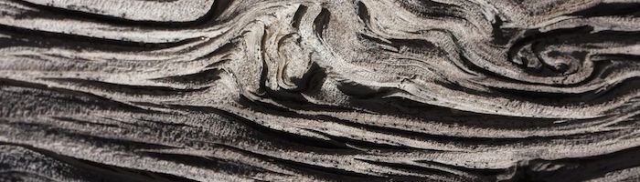
Like a painter who understands how the pigments of their paints work, the more we know about noise implementations the better we will be able to use them. For example, if we use a two dimensional noise implementation to rotate the space where straight lines are rendered, we can produce the following swirly effect that looks like wood. Again you can click on the image to see what the code looks like.

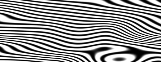
    pos = rotate2d( noise(pos) ) * pos; // rotate the space
    pattern = lines(pos,.5); // draw lines

Another way to get interesting patterns from noise is to treat it like a distance field and apply some of the tricks described in the Shapes chapter.

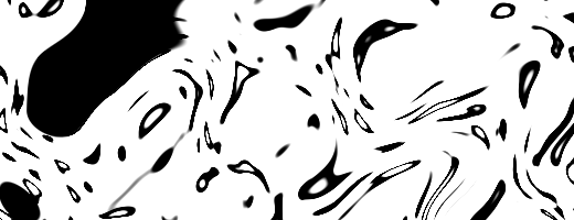
    color += smoothstep(.15,.2,noise(st*10.)); // Black splatter
    color -= smoothstep(.35,.4,noise(st*10.)); // Holes on splatter

A third way of using the noise function is to modulate a shape. This also requires some of the techniques we learned in the chapter about shapes.

For you to practice:

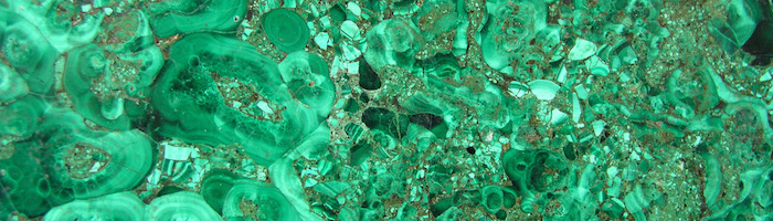
• What other generative pattern can you make? What about granite? marble? magma? water? Find three pictures of textures you are interested in and implement them algorithmically using noise.
• Use noise to modulate a shape.
• What about using noise for motion? Go back to the Matrix chapter. Use the translation example that moves the "+" around, and apply some random and noise movements to it.
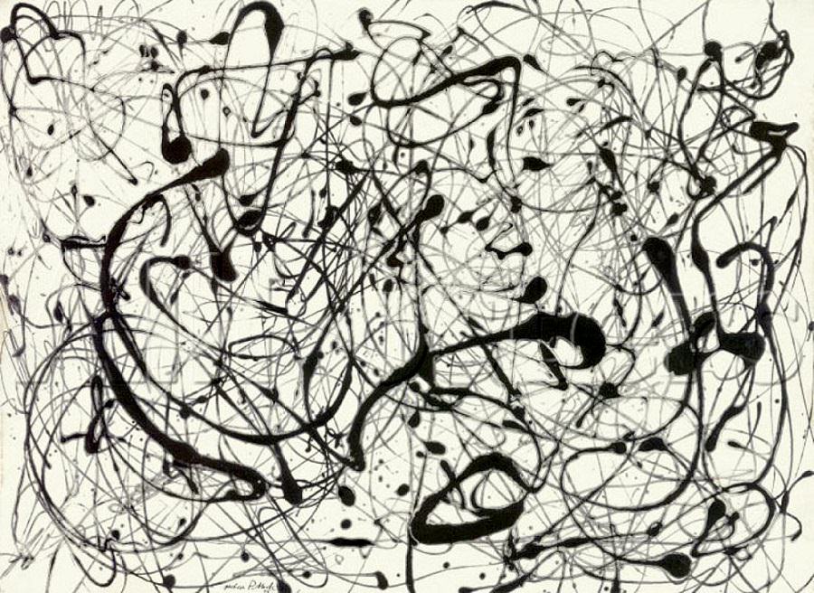
• Make a generative Jackson Pollock.

Improved Noise

An improvement by Perlin to his original non-simplex noise Simplex Noise, is the replacement of the cubic Hermite curve ( f(x) = 3x^2-2x^3 , which is identical to the smoothstep() function) with a quintic interpolation curve ( f(x) = 6x^5-15x^4+10x^3 ). This makes both ends of the curve more "flat" so each border gracefully stitches with the next one. In other words, you get a more continuous transition between the cells. You can see this by uncommenting the second formula in the following graph example (or see the two equations side by side here).

Note how the ends of the curve change. You can read more about this in Ken's own words.

Simplex Noise

For Ken Perlin the success of his algorithm wasn't enough. He thought it could perform better. At Siggraph 2001 he presented the "simplex noise" in which he achieved the following improvements over the previous algorithm:

• An algorithm with lower computational complexity and fewer multiplications.
• A noise that scales to higher dimensions with less computational cost.
• A noise without directional artifacts.
• A noise with well-defined and continuous gradients that can be computed quite cheaply.
• An algorithm that is easy to implement in hardware.

I know what you are thinking... "Who is this man?" Yes, his work is fantastic! But seriously, how did he improve the algorithm? Well, we saw how for two dimensions he was interpolating 4 points (corners of a square); so we can correctly guess that for three (see an implementation here) and four dimensions we need to interpolate 8 and 16 points. Right? In other words for N dimensions you need to smoothly interpolate 2 to the N points (2^N). But Ken smartly noticed that although the obvious choice for a space-filling shape is a square, the simplest shape in 2D is the equilateral triangle. So he started by replacing the squared grid (we just learned how to use) for a simplex grid of equilateral triangles.

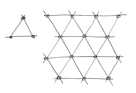
The simplex shape for N dimensions is a shape with N + 1 corners. In other words one fewer corner to compute in 2D, 4 fewer corners in 3D and 11 fewer corners in 4D! That's a huge improvement!

In two dimensions the interpolation happens similarly to regular noise, by interpolating the values of the corners of a section. But in this case, by using a simplex grid, we only need to interpolate the sum of 3 corners.

How is the simplex grid made? In another brilliant and elegant move, the simplex grid can be obtained by subdividing the cells of a regular 4 cornered grid into two isosceles triangles and then skewing it until each triangle is equilateral.

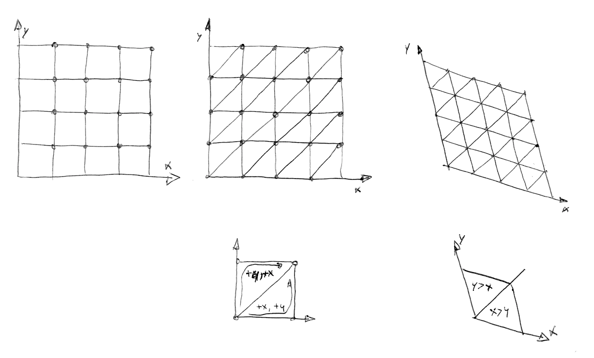
Then, as Stefan Gustavson describes in this paper: "...by looking at the integer parts of the transformed coordinates (x,y) for the point we want to evaluate, we can quickly determine which cell of two simplices that contains the point. By also comparing the magnitudes of x and y, we can determine whether the point is in the upper or the lower simplex, and traverse the correct three corner points."

In the following code you can uncomment line 44 to see how the grid is skewed, and then uncomment line 47 to see how a simplex grid can be constructed. Note how on line 22 we are subdividing the skewed square into two equilateral triangles just by detecting if x > y ("lower" triangle) or y > x ("upper" triangle).

All these improvements result in an algorithmic masterpiece known as Simplex Noise. The following is a GLSL implementation of this algorithm made by Ian McEwan and Stefan Gustavson (and presented in this paper) which is overcomplicated for educational purposes, but you will be happy to click on it and see that it is less cryptic than you might expect, and the code is short and fast.

Well... enough technicalities, it's time for you to use this resource in your own expressive way:

• Contemplate how each noise implementation looks. Imagine them as a raw material, like a marble rock for a sculptor. What can you say about the "feeling" that each one has? Squinch your eyes to trigger your imagination, like when you want to find shapes in a cloud. What do you see? What are you reminded of? What do you imagine each noise implementation could be made into? Following your guts and try to make it happen in code.

• Make a shader that projects the illusion of flow. Like a lava lamp, ink drops, water, etc.

• Use Simplex Noise to add some texture to a work you've already made.

In this chapter we have introduced some control over the chaos. It was not an easy job! Becoming a noise-bender-master takes time and effort.

In the following chapters we will see some well known techniques to perfect your skills and get more out of your noise to design quality generative content with shaders. Until then enjoy some time outside contemplating nature and its intricate patterns. Your ability to observe needs equal (or probably more) dedication than your making skills. Go outside and enjoy the rest of the day!

"Talk to the tree, make friends with it." Bob Ross

For your toolbox

• LYGIA's generative functions are a set of reusable functions to generate patterns in GLSL. It's a great resource to learn how to use randomness and noise to create generative art. It's very granular library, designed for reusability, performance and flexibility. And it can be easily be added to any projects and frameworks.