Cellular Noise
In 1996, sixteen years after Perlin's original Noise and five years before his Simplex Noise, Steven Worley wrote a paper called “A Cellular Texture Basis Function”. In it, he describes a procedural texturing technique now extensively used by the graphics community.
To understand the principles behind it we need to start thinking in terms of iterations. Probably you know what that means: yes, start using for loops. There is only one catch with for loops in GLSL: the number we are checking against must be a constant (const). So, no dynamic loops - the number of iterations must be fixed.
Let's take a look at an example.
Points for a distance field
Cellular Noise is based on distance fields, the distance to the closest one of a set of feature points. Let's say we want to make a distance field of 4 points. What do we need to do? Well, for each pixel we want to calculate the distance to the closest point. That means that we need to iterate through all the points, compute their distances to the current pixel and store the value for the one that is closest.
    float min_dist = 100.; // A variable to store the closest distance to a point

    min_dist = min(min_dist, distance(st, point_a));
    min_dist = min(min_dist, distance(st, point_b));
    min_dist = min(min_dist, distance(st, point_c));
    min_dist = min(min_dist, distance(st, point_d));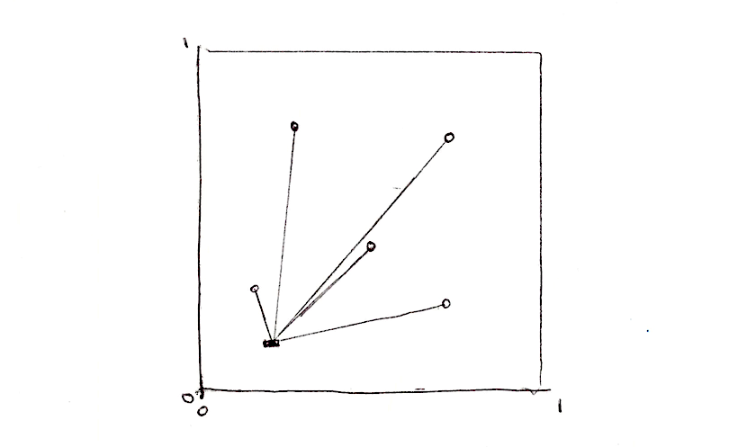
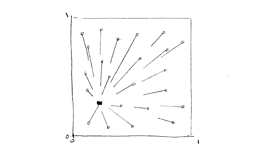
This is not very elegant, but it does the trick. Now let's re-implement it using an array and a for loop.
    float m_dist = 100.;  // minimum distance
    for (int i = 0; i < TOTAL_POINTS; i++) {
        float dist = distance(st, points[i]);
        m_dist = min(m_dist, dist);
    }
Note how we use a for loop to iterate through an array of points and keep track of the minimum distance using a min() function. Here's a brief working implementation of this idea:
In the above code, one of the points is assigned to the mouse position. Play with it so you can get an intuitive idea of how this code behaves. Then try this:
- How can you animate the rest of the points?
- After reading the chapter about shapes, imagine interesting ways to use this distance field!
- What if you want to add more points to this distance field? What if we want to dynamically add/subtract points?
Tiling and iteration
You probably notice that for loops and arrays are not very good friends with GLSL. Like we said before, loops don't accept dynamic limits on their exit condition. Also, iterating through a lot of instances reduces the performance of your shader significantly. That means we can't use this direct approach for large amounts of points. We need to find another strategy, one that takes advantage of the parallel processing architecture of the GPU.
One way to approach this problem is to divide the space into tiles. Not every pixel needs to check the distance to every single point, right? Given the fact that each pixel runs in its own thread, we can subdivide the space into cells, each one with one unique point to watch. Also, to avoid aberrations at the edges between cells we need to check for the distances to the points on the neighboring cells. That's the main brillant idea of Steven Worley's paper. At the end, each pixel needs to check only nine positions: their own cell's point and the points in the 8 cells around it. We already subdivide the space into cells in the chapters about: patterns, random and noise, so hopefully you are familiar with this technique by now.
    // Scale
    st *= 3.;

    // Tile the space
    vec2 i_st = floor(st);
    vec2 f_st = fract(st);
So, what's the plan? We will use the tile coordinates (stored in the integer coordinate, i_st) to construct a random position of a point. The random2f function we will use receives a vec2 and gives us a vec2 with a random position. So, for each tile we will have one feature point in a random position within the tile.
vec2 point = random2(i_st);Each pixel inside that tile (stored in the float coordinate, f_st) will check their distance to that random point.
    vec2 diff = point - f_st;
    float dist = length(diff);
The result will look like this:
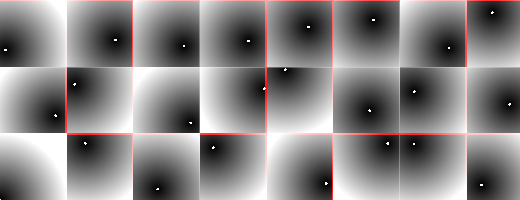
We still need to check the distances to the points in the surrounding tiles, not just the one in the current tile. For that we need to iterate through the neighbor tiles. Not all tiles, just the ones immediately around the current one. That means from -1 (left) to 1 (right) tile in x axis and -1 (bottom) to 1 (top) in y axis. A 3x3 region of 9 tiles can be iterated through using a double for loop like this one:
for (int y= -1; y <= 1; y++) {
    for (int x= -1; x <= 1; x++) {
        // Neighbor place in the grid
        vec2 neighbor = vec2(float(x),float(y));
        ...
    }
}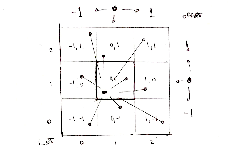
Now, we can compute the position of the points on each one of the neighbors in our double for loop by adding the neighbor tile offset to the current tile coordinate.
        ...
        // Random position from current + neighbor place in the grid
        vec2 point = random2(i_st + neighbor);
        ...
The rest is all about calculating the distance to that point and storing the closest one in a variable called m_dist (for minimum distance).
        ...
        vec2 diff = neighbor + point - f_st;

        // Distance to the point
        float dist = length(diff);

        // Keep the closer distance
        m_dist = min(m_dist, dist);
        ...
The above code is inspired by this article by Inigo's Quilez where he said:
"... it might be worth noting that there's a nice trick in this code above. Most implementations out there suffer from precision issues, because they generate their random points in "domain" space (like "world" or "object" space), which can be arbitrarily far from the origin. One can solve the issue moving all the code to higher precision data types, or by being a bit clever. My implementation does not generate the points in "domain" space, but in "cell" space: once the integer and fractional parts of the shading point are extracted and therefore the cell in which we are working identified, all we care about is what happens around this cell, meaning we can drop all the integer part of our coordinates away all together, saving many precision bits. In fact, in a regular voronoi implementation the integer parts of the point coordinates simply cancel out when the random per cell feature points are subtracted from the shading point. In the implementation above, we don't even let that cancelation happen, cause we are moving all the computations to "cell" space. This trick also allows one to handle the case where you want to voronoi-shade a whole planet - one could simply replace the input to be double precision, perform the floor() and fract() computations, and go floating point with the rest of the computations without paying the cost of changing the whole implementation to double precision. Of course, same trick applies to Perlin Noise patterns (but i've never seen it implemented nor documented anywhere)."
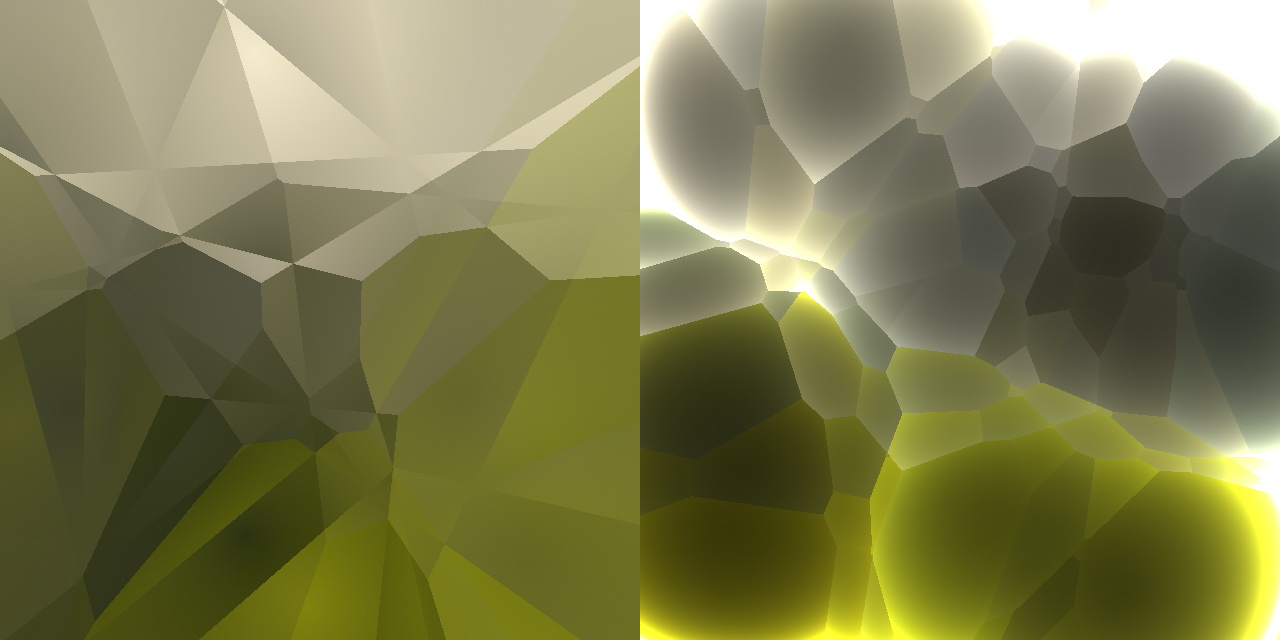
Recapping: we subdivide the space into tiles; each pixel will calculate the distance to the point in their own tile and the surrounding 8 tiles; store the closest distance. The result is a distance field that looks like the following example:
Explore this further by:
- Scaling the space by different values.
- Can you think of other ways to animate the points?
- What if we want to compute an extra point with the mouse position?
- What other ways of constructing this distance field can you imagine, besides
m_dist = min(m_dist, dist);? - What interesting patterns can you make with this distance field?
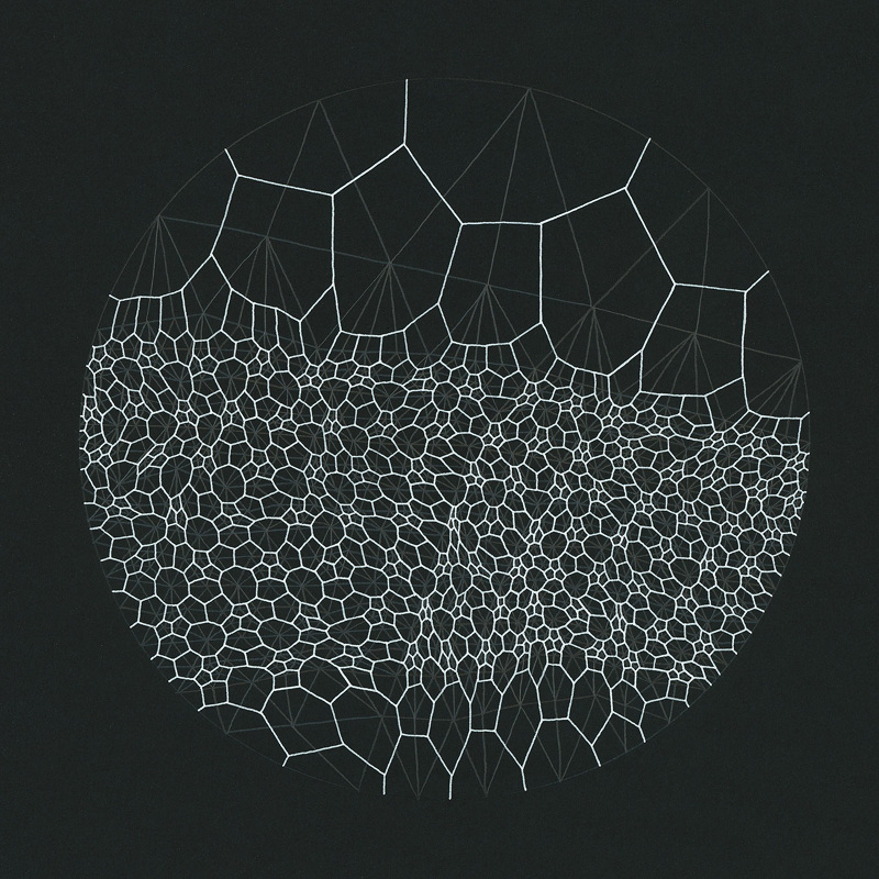
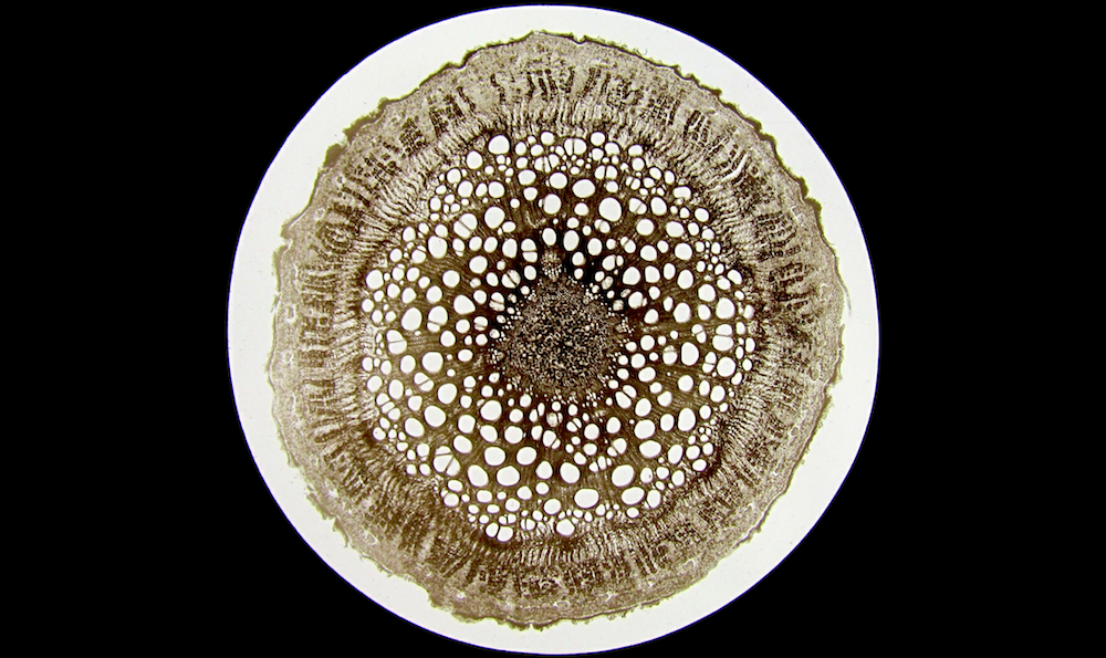
This algorithm can also be interpreted from the perspective of the points and not the pixels. In that case it can be described as: each point grows until it finds the growing area from another point. This mirrors some of the growth rules in nature. Living forms are shaped by this tension between an inner force to expand and grow, and limitations by outside forces. The classic algorithm that simulates this behavior is named after Georgy Voronoi.
Voronoi Algorithm
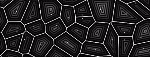
Constructing Voronoi diagrams from cellular noise is less hard than what it might seem. We just need to keep some extra information about the precise point which is closest to the pixel. For that we are going to use a vec2 called m_point. By storing the vector direction to the center of the closest point, instead of just the distance, we will be "keeping" a "unique" identifier of that point.
    ...
    if( dist < m_dist ) {
        m_dist = dist;
        m_point = point;
    }
    ...
Note that in the following code that we are no longer using min to calculate the closest distance, but a regular if statement. Why? Because we actually want to do something more every time a new closer point appears, namely store its position (lines 32 to 37).
Note how the color of the moving cell (bound to the mouse position) changes color according to its position. That's because the color is assigned using the value (position) of the closest point.
Like we did before, now is the time to scale this up, switching to Steven Worley's paper's approach. Try implementing it yourself. You can use the help of the following example by clicking on it. Note that Steven Worley's original approach uses a variable number of feature points for each tile, more than one in most tiles. In his software implementation in C, this is used to speed up the loop by making early exits. GLSL loops don't allow variable number of iterations, so you probably want to stick to one feature point per tile.
Once you figure out this algorithm, think of interesting and creative uses for it.
Improving Voronoi
In 2011, Stefan Gustavson optimized Steven Worley's algorithm to GPU by only iterating through a 2x2 matrix instead of 3x3. This reduces the amount of work significantly, but it can create artifacts in the form of discontinuities at the edges between the tiles. Take a look to the following examples.
Later in 2012 Inigo Quilez wrote an article on how to make precise Voronoi borders.
Inigo's experiments with Voronoi didn't stop there. In 2014 he wrote this nice article about what he calls voro-noise, a function that allows a gradual blend between regular noise and voronoi. In his words:
"Despite this similarity, the fact is that the way the grid is used in both patterns is different. Noise interpolates/averages random values (as in value noise) or gradients (as in gradient noise), while Voronoi computes the distance to the closest feature point. Now, smooth-bilinear interpolation and minimum evaluation are two very different operations, or... are they? Can they perhaps be combined in a more general metric? If that was so, then both Noise and Voronoi patterns could be seen as particular cases of a more general grid-based pattern generator?"
Now it's time for you to look closely at things, be inspired by nature and find your own take on this technique!
For your toolbox
- LYGIA's generative functions are a set of reusable functions to generate patterns in GLSL. It's a great resource to learn how to use randomness and noise to create generative art. It's very granular library, designed for reusability, performance and flexibility. And it can be easily be added to any projects and frameworks.